HoloViews 1.10 Release
We are very pleased to announce the release of HoloViews 1.10!
This release contains a large number of features and improvements. Some highlights include:
JupyterLab support:
- Full compatibility with JupyterLab when installing the jupyterlab_holoviews extension (#687)
New components:
Added
Sankeyelement to plot directed flow graphs (#1123)Added
TriMeshelement and datashading operation to plot small and large irregular meshes (#2143)Added
Chordelement to draw flow graphs between different nodes (#2137, #2143)Added
HexTileselement to plot data binned into a hexagonal grid (#1141)Added
Labelselement to plot a large number of text labels at once (as data rather than as annotations) (#1837)Added
Divelement to add arbitrary HTML elements to a Bokeh layout (#2221)Added
Violinelement to plot and compare distributions as kernel density estimates (#2114)Added
PointDraw,PolyDraw,BoxEdit, andPolyEditstreams to allow drawing, editing, and annotating glyphs on a Bokeh plot, and syncing the resulting data to Python (#2268)
Plus many other bug fixes, enhancements and documentation improvements. For full details, see the Release Notes.
If you are using Anaconda, HoloViews can most easily be installed by executing the command conda install -c pyviz holoviews . Otherwise, use pip install holoviews.
JupyterLab support
With JupyterLab now coming out of the alpha release stage, we have finally made HoloViews compatible with JupyterLab by creating the jupyterlab_pyviz extension. The extension can be installed with:
jupyter labextension install @pyviz/jupyterlab_pyviz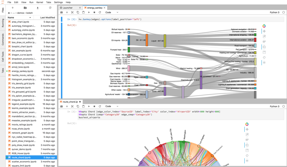
The JupyterLab extension provides all the interactivity of the classic notebook, and so both interfaces are now fully supported. Both classic notebook and JupyterLab now make it easier to work with streaming plots, because deleting or re-executing a cell in the classic notebook or JupyterLab now cleans up the plot and ensures that any streams are unsubscribed.
New elements
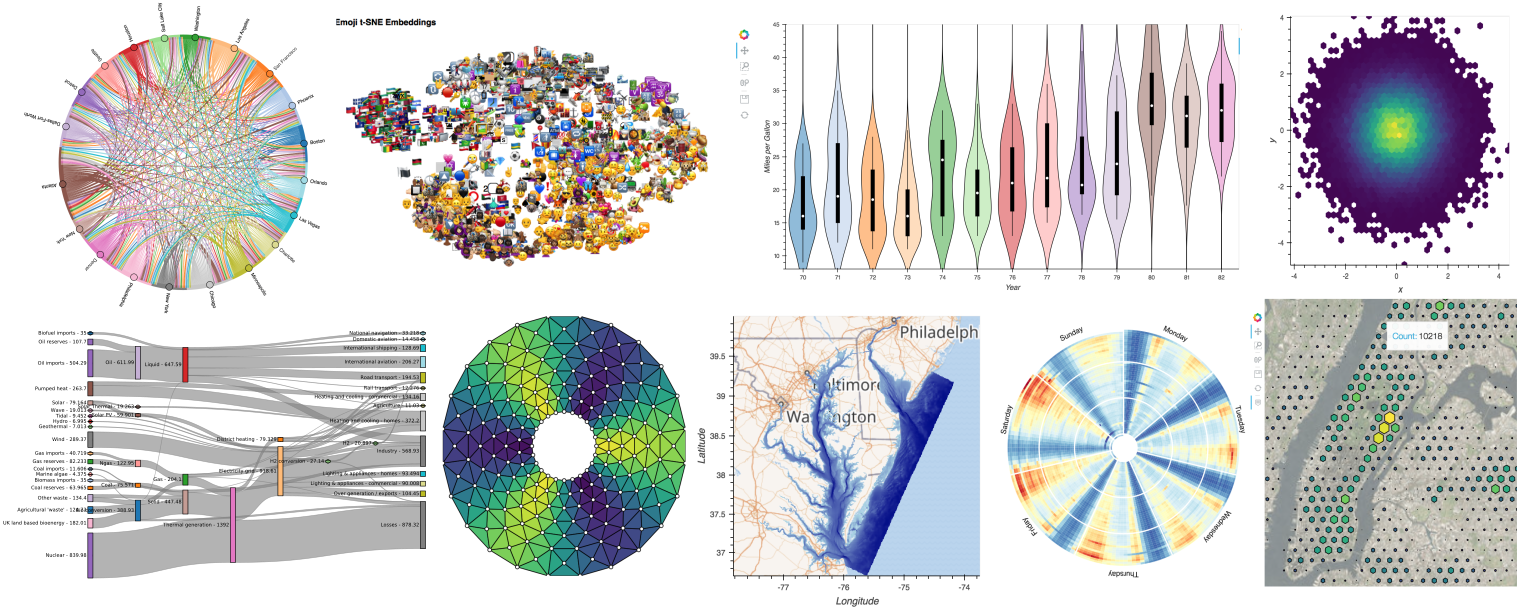
The main improvement in this release is the addition of a large number of elements. A number of these elements build on the Graph element introduced earlier in the 1.9 release, including the Sankey, Chord and TriMesh elements. Other new elements include HexTiles for binning many points on a hexagonal grid, Violins for comparing distributions across multiple variables, Labels for plotting large collections of text labels, and Div for displaying arbitrary HTML alongside Bokeh-based plots and tables.
Sankey
The new Sankey element is a pure-Python port of d3-sankey. Like most other elements, it can be rendered using both Matplotlib and Bokeh. In Bokeh, all the usual interactivity will be supported, such as providing hover information and interactively highlighting connected nodes and edges. Here we have rendered energy flow to SVG with matplotlib:

Chord
The Chord element had been requested a number of times, because it had previously been supported in the now deprecated Bokeh Charts package. Thanks to Bokeh's graph support, hovering and tapping on the Chord nodes highlights connected nodes, helping you make sense of even densely interconnected graphs:
TriMesh
Also building on the graph capabilities is the TriMesh element, which allows defining arbitrary meshes from a set of nodes and a set of simplices (triangles defined as lists of node indexes). The TriMesh element allows easily visualizing Delaunay triangulations and even very large meshes, thanks to corresponding support added to datashader. Below we can see an example of a TriMesh colored by vertex value and an interpolated datashaded mesh of the Chesapeake Bay containing 1M triangles:
HexTiles
Another often requested feature is the addition of a hexagonal bin plot, which can be very helpful in visualizing large collections of points. Thanks to the recent addition of a hex tiling glyph in the bokeh 0.12.15 release it was straightforward to add this support in the form of a HexTiles element, which supports both simple bin counts and weighted binning, and fixed or variable hex sizes.
Below we can see a HexTiles plot of ~7 million points representing the NYC population, where each hexagonal bin is scaled and colored by the bin value:
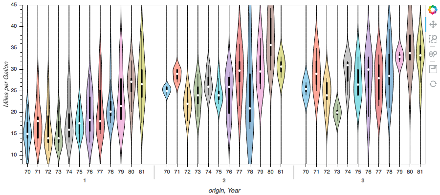
Violin
Violin elements have been one of the most frequently requested plot types since the Matplotlib-only Seaborn interface was deprecated from HoloViews. With this release a native implementation of violins was added for both Matplotlib and Bokeh, which allows comparing distributions across one or more independent variables:
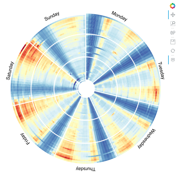
Radial HeatMap
Thanks to the contributions of Franz Woellert, the existing HeatMap element has now gained support for radial heatmaps. Radial heatmaps are useful for plotting quantities varying over some cyclic variable, such as the day of the week or time of day. Below we can see how the daily number of Taxi rides changes over the course of a year:
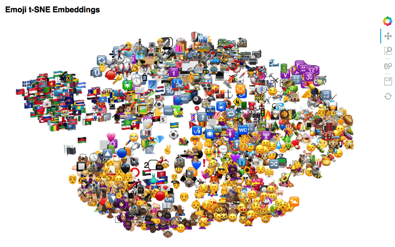
Labels
The existing Text element allows adding text to a plot, but only one item at a time, which is not suitable for plotting the large collections of text items that many users have been requesting. The new Labels element provides vectorized text plotting, which is probably most often used to annotate data points or regions of another plot type. Here we show that it can also be used on its own, to plot unicode emoji characters arranged by semantic similarity using the t-SNE dimensionality reduction algorithm:
Div
The Div element is exclusive to Bokeh and allows embedding arbitrary HTML in a Bokeh plot. One simple example of the infinite variety of possible uses for Div is to display Pandas summary tables alongside a plot:
bars + hv.Div(df.describe().to_html())
Editing Tools
In the Bokeh 0.12.15 release, a new set of interactive tools were added to edit and draw different glyph types. These tools are now available from HoloViews as the PointDraw, PolyDraw, BoxEdit, and PolyEdit streams classes, which make the drawn or edited data available to work with from Python. The drawing tools open up the possibility for very complex interactivity and annotations, allowing users to create even very complex types of interactive applications.
One example of the many workflows now supported is to draw regions of interest on an image using BoxEdit, computing the mean value over time for each such region:
Setting options
The new .options() method present on all viewable objects makes it much simpler to set options without worrying about the underlying difference between plot, style, and norm options. A comparison between the two APIs demonstrates how much more readable and easy to type the new approach is:
# New options API
img.options(cmap='RdBu_r', colorbar=True, width=360, height=300)

# Old opts API
img.opts(plot=dict(colorbar=True, width=360), style=dict(cmap='RdBu_r'));
Each option still belongs to one of the three categories internally, depending on whether it is processed by HoloViews or passed down into the underlying plotting library, but the user no longer usually has to remember which options are in which category.
It is also now possible to explicitly declare the backend for each option, which makes it easier to support multiple backends:
img.options(width=360, backend='bokeh').options(fig_inches=(6, 6), backend='matplotlib');
Image hover
Thanks to coming changes in bokeh 0.12.16, HoloViews will finally support hovering over images to reveal the underlying values, e.g. here we can see the NYC census data this time aggregated using datashader:
Data interfaces
The data interfaces that underlie HoloViews' ability to work natively with a variety of data structures also saw further improvements.
Binned and irregular data
It is now possible to declare binned data and irregular data, which has allowed Histogram and QuadMesh to finally support data interfaces. With this change, all Element types are now Dataset classes, with uniform architectures and supported usages.
## Binned data
n = 20
x = np.arange(n+1)         # Linear bins
y = np.logspace(0, 2, n+1) # Log bins
z = x*x[np.newaxis].T

# Irregular data
coords = np.linspace(-1.5, 1.5, n)
X,Y = np.meshgrid(coords, coords)

Qx = np.cos(Y) - np.cos(X) # 2D coordinate array
Qz = np.sin(Y) + np.sin(X) # 2D coordinate array
Z = np.sqrt(X**2 + Y**2)

hv.Histogram((x, y)) + hv.QuadMesh((y, x, z)) + hv.QuadMesh((Qx, Qz, Z))
import dask.array as da

n = 100
dask_array = da.from_array(np.random.rand(n, n), chunks=10)
hv.Image((range(n), range(n), dask_array))
Documentation & other improvements
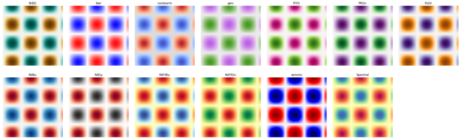
A new Colormap user guide provides an overview of the available colormaps and how to effectively choose a colormap to reveal your data. It also introduces the new hv.plotting.list_cmaps function, which makes it easy to query for a list of colormaps satisfying certain criteria (e.g. when providing a choice of appropriate colormaps to a user). For example, here is the output of hv.plotting.list_cmaps(category='Diverging', bg='light', reverse=False) when applied to an image, giving you a large number of alternatives that are all appropriate for this particular type of data:
An additional new Styling plots user guide provides an in-depth overview of how to control colors, cycles, palettes and cmaps, which are now consistently handled across backends and support new features such as discrete color_levels and symmetric color ranges:
img.options(color_levels=5, symmetric=True) + img.options(color_levels=11, symmetric=True)