GeoViews 1.5 Release
We are very pleased to announce the release of GeoViews 1.5!
This release contains a large number of features and improvements. Some highlights include:
Major feature:
- The bokeh backend now supports arbitrary geographic projections, no longer just Web Mercator (#170)
New components:
Added
Graphelement to plot networks of connected nodes (#115)Added
TriMeshelement and datashading operation to plot small and large irregular triangular meshes (#115)Added
QuadMeshelement and datashading operation to plot small and large, irregular rectilinear and curvilinear meshes (#116)Added
VectorFieldelement and datashading operation to plot small and large quiver plots and other collections of vectors (#122)Added
HexTileselement to plot data binned into a hexagonal grid (#147)Added
Labelselement to plot a large number of text labels at once (as data rather than as annotations) (#147)
New features:
Hover tool now supports displaying geographic coordinates as longitude and latitude (#158)
Added a new
geoviews.tile_sourcesmodule with a predefined set of tile sources (#165)Wrapped the xESMF library as a regridding and interpolation operation for rectilinear and curvilinear grids (#127)
HoloViews operations including
datashadeandrasterizenow retain geographiccrscoordinate system (#118)
Enhancements:
- Overhauled documentation and added a gallery (#121)
Plus many other bug fixes, enhancements and documentation improvements. For full details, see the Release Notes.
If you are using Anaconda, GeoViews can most easily be installed by executing the command conda install -c pyviz geoviews . Otherwise, you can also use pip install geoviews as long as you satisfy the cartopy dependency yourself.
Bokeh support for projections
In the past the Bokeh backend for GeoViews only supported displaying plots in Web Mercator coordinates. In this release this limitation was lifted and plots may now be projected to almost all supported Cartopy projections (to see the full list see the user guide):
cities = pd.read_csv(gv_path+'/cities.csv', encoding="ISO-8859-1")
points = gv.Points(cities[cities.Year==2050], ['Longitude', 'Latitude'], ['City', 'Population'])
features = gf.ocean * gf.land * gf.coastline

options = dict(width=600, height=350, global_extent=True,
               show_bounds=True, color='black', tools=['hover'], axiswise=True,
               color_index='Population', size_index='Population', size=0.002, cmap='viridis')

(features * points.options(projection=ccrs.Mollweide(), **options) +
 features * points.options(projection=ccrs.PlateCarree(), **options))
New elements
The other main enhancements to GeoViews in the 1.5 release come from the addition of a wide array of new elements, some of which were recently added in HoloViews and others which have been newly made aware of geographic coordinate systems and added to Geoviews.
Graph
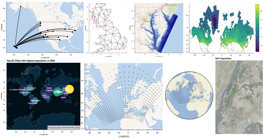
The first such addition is the new Graph element which was added to HoloViews 1.9 and has now been made aware of geographic coordinates. The example below (available in the gallery) demonstrates how to use the Graph element to display airport routes from Hawaii with great-circle paths:
VectorField
Another element that has been available in HoloViews and now been made aware of geographic coordinates is VectorField, useful for displaying vector quantities on a map. Like most HoloViews and GeoViews elements it can be rendered using both Bokeh (left) and Matplotlib (right):
TriMesh
Also building on the graph capabilities is the TriMesh element, which allows defining arbitrary meshes from a set of nodes and a set of simplices (triangles defined as lists of node indexes). The TriMesh element allows easily visualizing Delaunay triangulations and even very large meshes, thanks to corresponding support added to datashader. Below we can see a small TriMesh displayed as a wire frame and an interpolated datashaded mesh of the Chesapeake Bay containing 1M triangles:
QuadMesh
GeoViews has long had an Image element that supports regularly sampled, rectilinear meshes similar to matplotlib's imshow. To plot irregularly sampled rectilinear and curvilinear meshes, GeoViews now also has a QuadMesh element (akin to matplotlib's pcolormesh). Below is a curvilinear mesh loaded from xarray:
HexTiles
Another often requested feature is a hexagonal bin plot, which can be very helpful in visualizing large collections of points. Thanks to the recent addition of a hex tiling glyph in the bokeh 0.12.15 release it was straightforward to add this support in the form of a HexTiles element, which supports both simple bin counts and weighted binning, and fixed or variable hex sizes.
Below we can see a HexTiles plot of ~7 million points representing the NYC population, where each hexagonal bin is scaled and colored by the bin value:
Labels
The existing Text element allows adding text to a plot, but only one item at a time, which is not suitable for plotting the large collections of text items that many users have been requesting. The new Labels element provides vectorized text plotting, which is probably most often used to annotate data points or regions of another plot type. Here we select the 20 most populous cities in 2050, plot them using the Points element, and use the Labels element to label each point:
Features
Apart from the new collection of elements that were added, GeoViews 1.5 also comes with an impressive set of new features and enhancements.
Inbuilt Tile Sources
Since plotting on top of a map tile source is such a common and useful feature, a new tile_sources module has been added to GeoViews. The new geoviews.tile_sources module includes a number of commonly used tile sources from CartoDB, Stamen, ESRI, OpenStreetMap and Wikipedia, a small selection of which is shown below:
import geoviews.tile_sources as gvts

(gvts.CartoLight + gvts.CartoEco + gvts.ESRI + gvts.OSM + gvts.StamenTerrain + gvts.Wikipedia).cols(3)
Datashader & xESMF regridding
When working with mesh and raster data in a geographic context it is frequently useful to regrid the data. In this release we have improved support for regridding and rasterizing rectilinear and curvilinear grids and trimeshes using the Datashader and xESMF libraries. For a detailed overview of these capabilities see the user guide. As a quick summary:
- Datashader provides capabilities to quickly rasterize and regrid data of all kinds (
Image,RGB,HSV,QuadMesh,TriMesh,Path,PointsandContours) but does not support complex interpolation and weighting schemes - xESMF can regrid between general recti- and curvi-linear grids (
ImageandQuadMesh) with all ESMF regridding algorithms, such as bilinear, conservative and nearest neighbour
Below you can see the curvilinear mesh displayed above regridded and interpolated using xESMF:
Hover now displays lat/lon coordinates
As you may have noticed when hovering over some of the plots in this blog post, the hover tooltips now automatically format coordinates as latitudes and longitudes rather than the previous (and mostly useless) Web Mercator coordinates.
Operations now CRS aware
In the past when operations defined in HoloViews were applied to GeoViews elements, the coordinate reference system (CRS) of the data was ignored and a HoloViews element was returned. Thanks to the ability to register pre- and post-processors for operations, operations such as datashade, rasterize, contours and bivariate_kde will now retain the coordinate system of the data.
As a simple example we will use the bivariate_kde operation from HoloViews to generate a density map from a set of points. Here the PlateCarree crs is retained throughout the operation so that the returned Contours element is appropriately projected on top of the tile source:
from holoviews.operation.stats import bivariate_kde

population = gv.Points(cities[cities.Year==2050], ['Longitude', 'Latitude'], 'Population')

gvts.StamenTerrainRetina * bivariate_kde(population, bandwidth=0.1).options(
    width=500, height=450, show_legend=False, is_global=True
).relabel('Most populous city density map')
Projection operation improved
The gv.project operation provides a high-level wrapper for projecting all GeoViews element types and now has better handling for polygons and paths as well as all the new element types added in this release.
Improved documentation & gallery
This release was also accompanied by an overhaul of the existing documentation, specifically an improved user guide on projections and a whole new gallery with a wide (and expanding) selection of examples.